

Cassini MIMI Investigation at Fundamental Technologies
Numerical Computation of Energy-Dependent Geometric Factors of E and F Electron Detectors of CASSINI/MIMI/LEMMS
Technical Report by Xiaodong Hong and Thomas P. Armstrong, May 10, 1997
Chapter 2 Calculation of Magnetic Field of the Cassini/MIMI/LEMMS Sensor
Assuming that the magnetization of a rectangular surface is uniformly polarized at the normal direction, one can obtain the analytic expression of the magnetic field produced by a rectangular magnet. The magnet is located in the plane defined by -a <= x <=+a, -b<=y<=+b, z=0. z is the direction of magnetization, which one can obtain [1,2] thus:
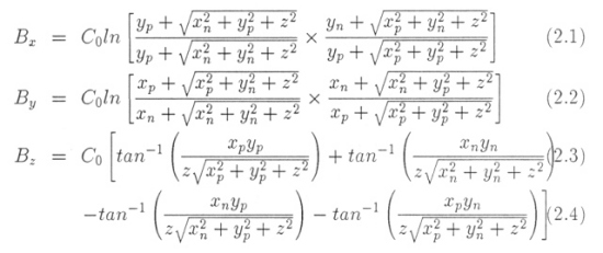
where xp=x+a, xn=x-a, yp=y+b, yn=y-b.
The measured magnetic field in the Cassini/MIMI/LEMMS is given for the midplane of the aperture. Therefore, we adopt aperture coordinates for use in the trajectory calculations and must express the field as from a superposition of pairs of uniformly magnetized sources. These have been displaced from the z=0 plane by a distance of +/- d/2 and then rotated by +/-14.7º around the x axis. Because the magnetic field in the LEMMS aperture is produced by a pair of magnetized slabs that are displaced from the midplane and tilted in order to achieve a variation of field strength, we need to express the field of an individual slab in coordinates that are convenient for the entire aperture assembly. Hence, each slab must be displaced and tilted for its contribution to the total field.
In order to use the above analytic expressions we divide each slab into smaller pieces, with each piece pairing with the other piece of the other slab. The following steps show the calculation of the magnetic field of a pair of rectangular magnets. Then we can sum up all the magnetic fields produced by all the pairs of magnets to obtain the total field strength produced by the slabs.
Translation of the first magnetic coordinates:
|
x0=x-x1 |
(2.5) |
|
y0=y-y1 |
(2.6) |
|
z0=z+z1 |
(2.7) |
The rotation of the first magnetic slab coordinates:
|
x'1=x0 |
(2.8) |
| y'1=-y0 cos Φ - z0 sin Φ |
(2.9) |
| z'1=y0 sin Φ - z0 cos Φ |
(2.10) |
Next the rotation of the coordinates in the second magnetic slab:
|
x'2=x0 |
(2.11) |
| y'2=y0 cos Φ - (z0-d) sin Φ |
(2.12) |
| z'2=y0 sin Φ + (z0-d) cos Φ |
(2.13) |
where d is the separation between two slabs, and x1, y1, and z1 are the distances translated from the first slab to the original coordinates.
The inverse rotation of the magnetic field must be performed so that B1, B2 can be added up correctly. For slab #1:
|
Bx10=Bx1 |
(2.14) |
| By10=-By1 cos Φ + Bz1 sin Φ |
(2.15) |
| Bz10=-By1 sin Φ - Bz1 cos Φ |
(2.16) |
where Bx1, By1, Bz1 are components in the x'1y'1z'1 coordinate system. Bx10, By10, Bz10 are components in the aperture coordinate system. For slab #2:
|
Bx20=Bx2 |
(2.17) |
| By20=By2 cos Φ + Bz2 sin Φ |
(2.18) |
| Bz20=-By2 sin Φ + Bz2 cos Φ |
(2.19) |
where Bx2, By2, Bz2 are components in the x'2y'2z'2 coordinate system. Bx20, By20, Bz20 are components in the aperture coordinate system.
Modification of the coordinate transformations has been made according to equations 2.5 - 2.13. The magnetic fields are represented in the slab coordinates and added up after inverse rotation (equations 2.14 - 2.19) of the coordinates.
Due to the symmetry, Bx, By should be zeroes at the z=0 plane. This is proved in Wu's model calculation with the inverse rotation.
The measurement of the magnetic field produced by the magnets of Cassini/MIMI/LEMMS is given in table 1 (Livi, Lagg et al., 1996). The z components of the magnetic field are measured at the z=0 plane at various x and y positions and at the y=2.85 cm plane for some x and z positions.
The simulation of the magnetic field produced by the magnets is done according to the Wu, McKee, Armstrong [1] model discussed earlier. The normalization of the calculation values is done according to the maximum values of the measurement. The calculation, absolute difference, and relative difference values are given in tables 2.2 - 2.4 at various x, y, and z positions with the Wu, McKee, Armstrong coordinates applied to Galileo LEMMS.
There is also a slightly improved version of the simulation of the magnetic field which provides a better fit for the open aperture area (see figure 2.6). This is achieved by adding a small negative magnet strip near the open aperture (see FDMOD6.CMN in Appendix D for reference). Both simulations of the magnetic field are used in the trajectory tracing to obtain the geometric factors of the Cassini/MIMI/LEMMS E and F detectors. Other plots of the improved simulation of the magnetic field are shown in figures 2.7 - 2.10.
Figures:
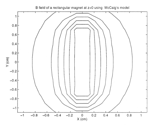 |
Figure 2.1 The contour of the magnetic field produced by a rectangular slab with a=0.15 cm and b=0.8 cm. |
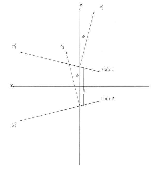 |
Figure 2.2 The locations of the two magnetic slabs. |
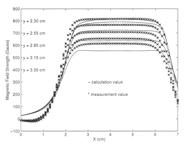 |
Figure 2.3 Comparison of the calculated vs. measured values of the magnetic field at z=0 cm of various y. |
 |
Figure 2.4 Contour of the calculated magnetic field at z=0 cm. |
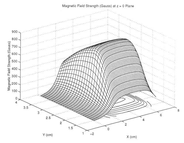 |
Figure 2.5 The mesh and contour of the calculated magnetic field at z=0 cm. |
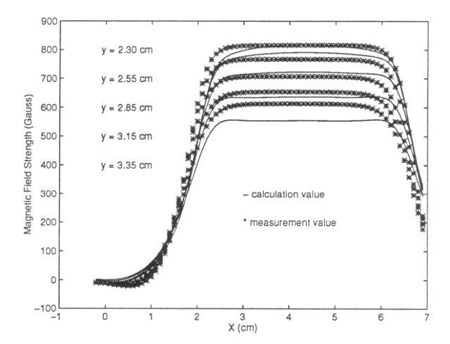 |
Figure 2.6 Comparison of the improved calculated vs. measured values of magnetic field at z=0 cm of various y. |
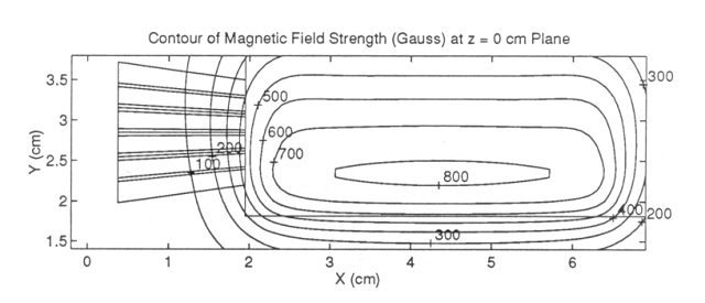 |
Figure 2.7 Contour of the improved calculated magnetic field at z=0 cm. |
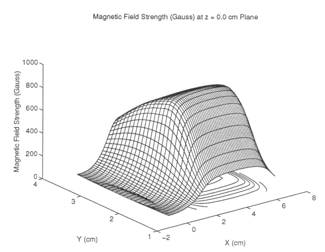 |
Figure 2.8 The mesh and contour of the improved calculated magnetic field at z=0 cm. |
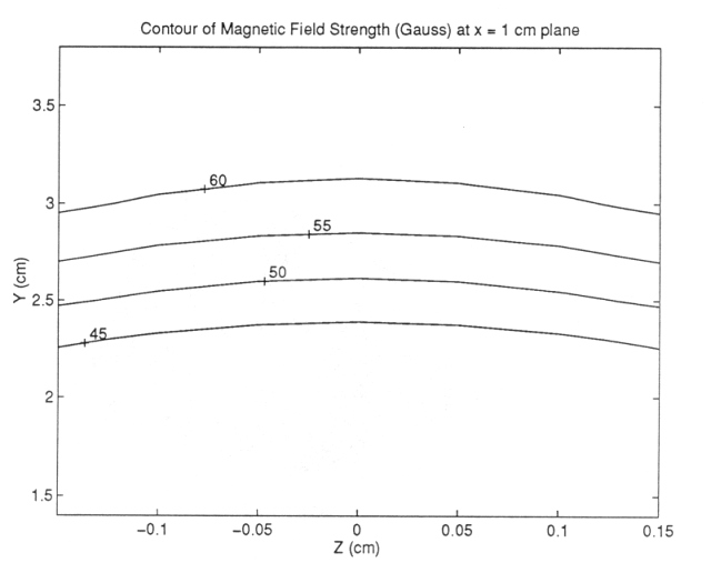 |
Figure 2.9 Contour of the improved calculated magnetic field at x=1 cm plane. |
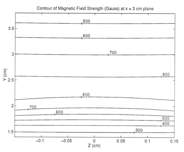 |
Figure 2.10 Contour of the improved calculated magnetic field at x=3 cm plane. |
Table 2.1
Table 2.2
Table 2.3
Table 2.4
Next: Chapter 3 Computation of Geometric Factors
Return to Technical Report Table of Contents
Return to Cassini
MIMI table of contents page.
Return to Fundamental
Technologies Home Page.
Updated 8/8/19, Cameron Crane
QUICK FACTS
Mission Duration: The Cassini-Huygens mission launched on October 15 1997, and ended on September 15 2017.
Destination: Cassini's destination was Saturn and its moons. The destination of the Huygens Probe's was Saturn's moon Titan.
Orbit: Cassini orbited Saturn for 13 years before diving between its rings and colliding with the planet on September 15th, 2017.